Creating a high-order finite volume transport scheme
Over the last year of my PhD I have been working to create a finite volume transport scheme, called ‘cubicFit’, that is second-order convergent on arbitrary meshes. Recently, I have tried modifying the cubicFit transport scheme to obtain high-order convergence: that is, convergence greater than second-order. Here I'll introduce a one-dimensional version of the cubicFit scheme and explain how it can be modified to obtain high-order convergence.
One-dimensional finite volume approximation
To formulate the one-dimensional cubicFit transport scheme, I'll start from the transport equation for a dependent variable \(\phi\) assuming a non-negative velocity \(u\) that is constant in time and space, \begin{equation} \frac{\partial \phi}{\partial t} = - u \frac{\partial \phi}{\partial x} \label{eqn:transport} \end{equation} where the term on the right-hand side is called the flux divergence. With a C-grid staggering, velocity values are stored at faces and \(\phi\) values are stored at cell centres. Using the finite volume method to discretise the flux divergence term, equation \eqref{eqn:transport} becomes \begin{equation} \frac{\partial \phi}{\partial t} = - u \frac{\phi_R - \phi_L}{\Delta x} \label{eqn:fluxdiv} \end{equation} where \(\phi_L\) and \(\phi_R\) are approximate values of \(\phi\) at the left and right faces respectively, and \(\Delta x\) is the distance between the faces.
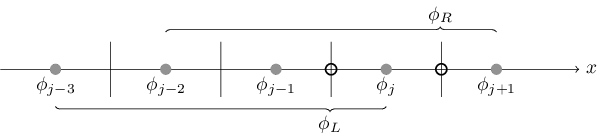
The cubicFit scheme approximates a face value using four neighbouring cell centre values, as shown above. For each face, a cubic polynomial is found that interpolates the four data points, \begin{equation} \phi = a_1 + a_2 x + a_3 x^2 + a_4 x^3 \text{.} \label{eqn:cubic} \end{equation} By choosing a local coordinate with its origin at the face then the value of \(\phi\) at the face is just \(a_1\), which is calculated as follows. Assuming a uniform mesh with \(\Delta x = 1\) and choosing the position of \(\phi_{i+1/2}\) to be \(x=0\), equation \eqref{eqn:cubic} is evaluated at the cell centres \(\phi_{i-2}, \ldots, \phi_{i+1}\) to form the matrix equation \begin{align} \mathbf{B} \mathbf{a} &= \mathbf{\phi} \\ \begin{bmatrix} 1 & -5/2 & 25/4 & -125/8 \\ 1 & -3/2 & 9/4 & -27/8 \\ 1 & -1/2 & 1/4 & -1/8 \\ 1 & 1/2 & 1/4 & 1/8 \\ \end{bmatrix} \begin{bmatrix} a_1 \\ a_2 \\ a_3 \\ a_4 \end{bmatrix} &= \begin{bmatrix} \phi_{i-2} \\ \phi_{i-1} \\ \phi_i \\ \phi_{i+1} \end{bmatrix} \text{.} \end{align} The unknown coefficients \(\mathbf{a}\) are found by inverting \(\mathbf{B}\) such that \(\mathbf{a} = \mathbf{B}^{-1} \mathbf{\phi}\). The inverse matrix is \begin{align} \mathbf{B}^{-1} = \frac{1}{48} \begin{bmatrix} 3 & -15 & 45 & 15 \\ 2 & -6 & -42 & 46 \\ -12 & 60 & -84 & 36 \\ -8 & 24 & -24 & 8 \end{bmatrix} \label{eqn:cubicfit-inverse} \end{align} Since \(x=0\) was chosen to be the position \(i+1/2\) then \begin{align} \phi_{i+1/2} = a_1 = \frac{1}{16} \begin{bmatrix} 1 \\ -5 \\ 15 \\ 5 \end{bmatrix} \cdot \begin{bmatrix} \phi_{i-2} \\ \phi_{i-1} \\ \phi_i \\ \phi{i+1} \end{bmatrix} \text{.} \label{eqn:cubicfit-fluxcoeffs} \end{align}
One-dimensional finite difference approximation
To obtain a high-order version of the one-dimensional cubicFit transport scheme I return to the flux divergence term on the right-hand side of equation \eqref{eqn:transport} and discretise it using the finite difference method. Using this method, the flux divergence of cell \(i\) is calculated using a cubic approximation using cell centre values \(\phi_{i-2}, \ldots, \phi_{i+1}\). A matrix equation is constructed using equation \eqref{eqn:cubic} evaluated at every cell centre. For convenience, assume that \(\Delta x = 1\) and that \(x=0\) at the cell centre position of \(\phi_i\), hence the matrix equation becomes \begin{align} \mathbf{B} \mathbf{a} &= \mathbf{\phi} \\ \begin{bmatrix} 1 & -2 & 4 & -8 \\ 1 & -1 & 1 & -1 \\ 1 & 0 & 0 & 0\\ 1 & 1 & 1 & 1\\ \end{bmatrix} \begin{bmatrix} a_1 \\ a_2 \\ a_3 \\ a_4 \end{bmatrix} &= \begin{bmatrix} \phi_{i-2} \\ \phi_{i-1} \\ \phi_i \\ \phi_{i+1} \end{bmatrix} \end{align} The unknown coefficients \(\mathbf{a}\) are found by calculating the inverse matrix, \begin{align} \mathbf{B}^{-1} = \frac{1}{6} \begin{bmatrix} 0 & 0 & 6 & 0 \\ 1 & -6 & 3 & 2 \\ 0 & 3 & -6 & 3 \\ -1 & 3 & -3 & 1 \end{bmatrix} \text{.} \end{align} To calculate the flux divergence I calculate the derivative \(\partial \phi / \partial x = a_2 + 2 a_3 x + 3 a_4 x^2\). Evaluating the flux divergence at \(\phi_i\) where \(x=0\) then \(\partial \phi_i / \partial x = a_2\). Hence I find that the finite difference weighted sum is \begin{align} -u \frac{\partial \phi_i}{\partial x} = -u a_2 = -u \cdot \frac{1}{6} \begin{bmatrix} 1 \\ -6 \\ 3 \\ 2 \end{bmatrix} \cdot \begin{bmatrix} \phi_{i-2} \\ \phi_{i-1} \\ \phi_i \\ \phi_{i+1} \end{bmatrix} \label{eqn:fd-fluxdiv} \end{align} The cubic finite difference approximation given in equation \eqref{eqn:fd-fluxdiv} is conservative on uniform meshes. This can be demonstrated by decomposing the weights vector, \begin{align} -u \cdot \frac{1}{6} \begin{bmatrix} 1 \\ -6 \\ 3 \\ 2 \end{bmatrix} \cdot \begin{bmatrix} \phi_{i-2} \\ \phi_{i-1} \\ \phi_i \\ \phi_{i+1} \end{bmatrix} &= -u \cdot \frac{1}{6} \left( \begin{bmatrix} 0 \\ -1 \\ 5 \\ 2 \end{bmatrix} - \begin{bmatrix} -1 \\ 5 \\ 2 \\ 0 \end{bmatrix} \right) \cdot \begin{bmatrix} \phi_{i-2} \\ \phi_{i-1} \\ \phi_i \\ \phi_{i+1} \end{bmatrix} \\ &= -u \left( \frac{1}{6} \begin{bmatrix} -1 \\ 5 \\ 2 \end{bmatrix} \cdot \begin{bmatrix} \phi_{i-1} \\ \phi_i \\ \phi_{i+1} \end{bmatrix} - \frac{1}{6} \begin{bmatrix} -1 \\ 5 \\ 2 \end{bmatrix} \cdot \begin{bmatrix} \phi_{i-2} \\ \phi_{i-1} \\ \phi_i \end{bmatrix} \right) \text{.} \label{eqn:fd-fluxcoeffs} \end{align} Notice that the flux divergence has been rewritten as the difference between right and left fluxes as in equation \eqref{eqn:fluxdiv}.
High-order correction in one dimension
The high-order correction to the cubicFit scheme is calculated as the difference between the cubic finite difference approximation (equation \ref{eqn:fd-fluxcoeffs}) and the uncorrected cubicFit approximation (equation \ref{eqn:cubicfit-fluxcoeffs}), \begin{align} \mathrm{correction}(\phi_{i+1/2}) &= \left( \frac{1}{6} \begin{bmatrix} 0 \\ -1 \\ 5 \\ 2 \end{bmatrix} - \frac{1}{16} \begin{bmatrix} 1 \\ -5 \\ 15 \\ 5 \end{bmatrix} \right) \cdot \begin{bmatrix} \phi_{i-2} \\ \phi_{i-1} \\ \phi_i \\ \phi_{i+1} \end{bmatrix} \\ &= \frac{1}{48} \begin{bmatrix} -3 \\ 7 \\ -5 \\ 1 \end{bmatrix} \cdot \begin{bmatrix} \phi_{i-2} \\ \phi_{i-1} \\ \phi_i \\ \phi_{i+1} \end{bmatrix} \label{eqn:correction} \end{align} which can be decomposed into a linear combination of second derivatives where \(\partial_x^2 \phi_i = \phi_{i-1} - 2 \phi_i + \phi_{i+1}\), \begin{align} &= \frac{1}{48} \left( -3 \begin{bmatrix}1 \\ -2 \\ 1 \\ 0\end{bmatrix} + \begin{bmatrix}0 \\ 1 \\ -2 \\ 1\end{bmatrix} \right) \cdot \begin{bmatrix} \phi_{i-2} \\ \phi_{i-1} \\ \phi_i \\ \phi_{i+1} \end{bmatrix} \\ &= \frac{1}{48} \left( -3 \partial_x^2 \phi_{i-1} + \partial_x^2 \phi_i \right) \text{.} \end{align} Applying this correction using the three-point approximation of the second derivative results in third-order convergence on uniform meshes and second-order convergence on non-uniform meshes.
Alternatively, the second derivative can be calculated from equation \eqref{eqn:cubic} such that \(\partial_x^2 \phi = 2a_3 + 6a_4x\) where \(a_3\) and \(a_4\) can be calculated using equation \eqref{eqn:cubicfit-inverse}. This approach results in fourth-order convergence on uniform meshes and second-order convergence on non-uniform meshes, as seen in the convergence plot above. Curiously, this approach yields the correction \begin{align} \mathrm{correction}(\phi_{i+1/2}) &= \frac{1}{48} \left( -3 \cdot \begin{bmatrix} 0 \\ 1 \\ -2 \\ 1 \end{bmatrix} + \begin{bmatrix} -1 \\ 4 \\ -5 \\ 2 \end{bmatrix} \right) \cdot \begin{bmatrix} \phi_{i-2} \\ \phi_{i-1} \\ \phi_i \\ \phi_{i+1} \end{bmatrix} \\ &= \frac{1}{48} \cdot \begin{bmatrix} -1 \\ 1 \\ 1 \\ -1 \end{bmatrix} \cdot \begin{bmatrix} \phi_{i-2} \\ \phi_{i-1} \\ \phi_i \\ \phi_{i+1} \end{bmatrix} = \frac{1}{48} \left( \begin{bmatrix} -1 \\ 2 \\ -1 \\ 0 \end{bmatrix} + \begin{bmatrix} 0 \\ -1 \\ 2 \\ -1 \end{bmatrix} \right) \cdot \begin{bmatrix} \phi_{i-2} \\ \phi_{i-1} \\ \phi_i \\ \phi_{i+1} \end{bmatrix} \\ &= -\frac{1}{48} \left( \partial_x^2 \phi_{i-1} + \partial_x^2 \phi_i \right) \cdot \begin{bmatrix} \phi_{i-2} \\ \phi_{i-1} \\ \phi_i \\ \phi_{i+1} \end{bmatrix} \text{.} \end{align}
Can high-order be obtained in two dimensions?
The one-dimensional version of cubicFit exactly interpolates four data points with a cubic polynomial. However, on a two-dimensional mesh of rectangular cells, the stencil has four points in the \(x\) direction and three points in the \(y\) direction for a total of twelve data points. The multidimensional polynomial is then $$ \phi = a_1 + a_2 x + a_3 y + a_4 x^2 + a_5 xy + a_6 y^2 + a_7 x^3 + a_8 x^2 y + a_9 x y^2 \text{.} $$ Hence, we have an overconstrained system of equations with twelve data points and nine unknown coefficients \(a_1 \ldots a_9\) which is solved using a least-squares approach.
In two dimensions, it is no longer clear to me how to formulate a high-order correction, but Skamarock and Gassmann 2011 used their one-dimensional high-order correction in two dimensions by applying it at each cell face. It seems to me that their approach could be applied to cubicFit, though I have yet to have success applying a high-order correction to the OpenFOAM cubicFit implementation for arbitrarily-structured meshes. I hope to describe the features of this scheme in a future post.